
Summer ☀️ is here, and so we’re back with our reading club at the Saale river! In this session, we dive into the fascinating world of entropy—a concept that lies at the heart of thermodynamics and statistical mechanics. A deeper understanding of entropy emerged through the work of Max Planck, who applied the ideas of Ludwig Boltzmann to light. This connection helped reveal the microscopic foundations of entropy through the quantization of energy. In our reading, we explore the shelf model by Arnd H. Jungermann to develop an intuitive understanding of the relationship between entropy and other fundamental concepts such as energy, heat, and temperature.

Reading at Strand 22 at the Saale river in the Paradies park in Jena.
When we think of entropy, two words often come to mind: randomness and disorder. We usually say that a system has low entropy when its energy is well organized and can readily be used to perform work. In contrast, a system has high entropy when its energy becomes more evenly and randomly distributed, leaving no energy gradients available to drive useful work.
While these descriptions are intuitive, they do not provide a physical picture of what entropy actually represents. To address this, Jungermann introduced the shelf model, a simple yet powerful analogy that helps visualize entropy from a molecular, quantum physical perspective. Surprisingly, the model is based on something very familiar—a shelf, like the one we use every day to store books or other household items.
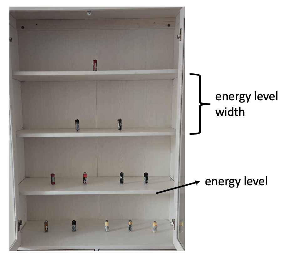
Objects occupying different shelves of a wardrobe
(after Jungermann, 2006)
1. What is the Shelf model?
We can understand the shelf model by comparing it to the construction of a wardrobe. The vertical side panels of the wardrobe can be viewed as an energy scale, while the shelves represent the allowed molecular energy levels. When building a wardrobe, shelves can only be installed at specific positions along the vertical panels. Similarly, in quantum mechanics, a molecule can occupy only certain discrete energy levels; the energy difference between them is not arbitrary.
Each shelf therefore represents one allowed energy level of the molecule or system under study. Different molecules have different sets of allowed energy levels. The number of shelves, their spacing, and their positions are not universal, but depend on the specific molecule. The lowest shelf (the ground state) also does not need to occur at the same height for every molecule. Each molecule has its own characteristic energy spectrum. However, within a given molecule, the higher the shelf, the greater the corresponding energy of that state.
Now, let us fill these shelves with ten particles with each particle of being one energy unit (1eu). These particles can be distributed in several ways shown in Figure below with the where ni is the number of particles at the i-th shelf or energy level, and N is the total number of particles (ten in this case), where Ei is the energy level of the i-th shelf.
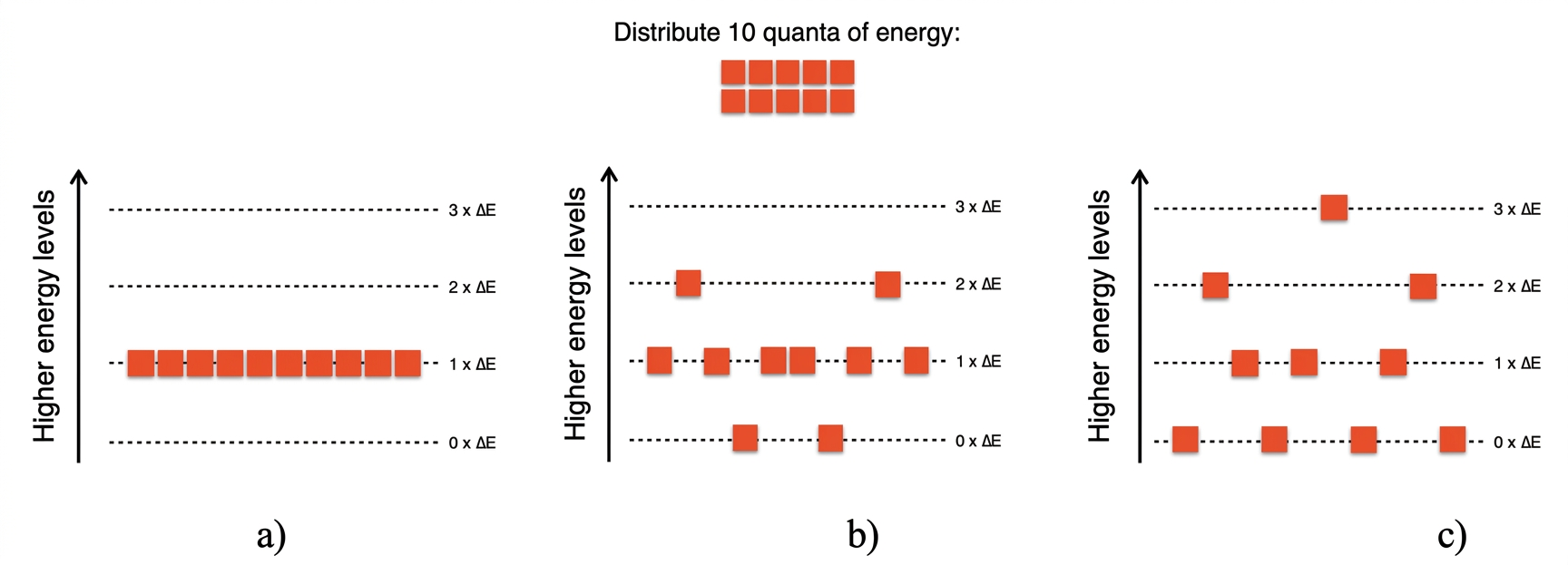
Illustration of distributing 10 quanta of energy
over 4 equally spaced energy levels.
The way particles are distributed among the energy shelves defines the macrostate of the system. In this example, there are three possible macrostates, each corresponding to a different distribution of particles across the shelves. Each macrostate can be realized through many different microstates. A microstate specifies the exact arrangement of individual particles, whereas a macrostate only specifies how many particles occupy each energy shelf. The number of microstates corresponding to a given macrostate can be calculated statistics: W = N! / n1! * n2! * n3! … ni!. The numerator, N!, represents all possible arrangements of the particles. Assume the particles are labeled, however, exchanging particles that occupy the same energy shelf do not produce a new microstate, so basically the order of particles within a shelf is not important. Therefore, we divide by the factorial of the number of particles on each shelf to eliminate these duplicate arrangements. During this counting, the occupation number of each shelf (the number of particles on that shelf) remains fixed.
For the three states shown in the Figure, we have:
- Macrostate A: all particles occupy the second shelf. The number of microstates is WA= ,
- Macrostate B: two particles occupy the lowest shelf, six particles occupy the second shelf and remaining two occupy the third shelf. The number of microstates is WB =
- Macrostate C: the number of microstates is WC =
Among all possible macrostates, the one with the largest number of microstates is the most probable and is therefore the state that is most likely to be observed in reality. In this example, macrostate C has the largest number of microstates.
Boltzmann related entropy to the number of accessible microstates through the equation: S = kB ln W, where kB is the Boltzmann constant and W is the number of microstates. Consequently, a macrostate with a larger number of microstates has a higher entropy. This provides a statistical interpretation of the second law of thermodynamics: systems naturally evolve toward the macrostate with the greatest number of accessible microstates because it is the most probable.
2. Three rules to understand entropy variations
The shelf model of entropy provides an intuitive way to understand measured values of entropy and entropy changes. These variations can be explained using three rules proposed by Jungermann. Throughout the model, it is assumed that the energy levels (or shelves) are equally spaced.
The first rule, the Basic Rule, describes how the total energy is distributed among the available energy levels. According to this rule, the energy is distributed such that the largest possible number of energy levels is occupied, while at the same time keeping the occupied levels as low in energy as possible. Consequently, entropy can be viewed as a measure of the number of microstates. This basic rule referred by Jungerman, is the qualitative consequence of maximising the total number of microstates (or the entropy), which makes the higher occupancy of energy levels progressively less probable (following the Boltzmann distribution).
The second rule, the Force Rule, concerns the strength of the forces acting on the particles. When particles are held together by strong intermolecular or interatomic forces, they are confined to a smaller region of space. As a result, the spacing between the allowed energy levels increases, and the energy required for a quantum leap (a transition between two discrete energy levels) becomes larger. This explains why solids generally have lower entropy than liquids or gases, because the particles experience weaker constraints and can access a larger number of energy levels.
The third rule, the Mass Rule, relates entropy to the mass of the particles. As the mass of a particle increases, the spacing between adjacent energy levels decreases, making quantum transitions possible with smaller amounts of energy. Consequently, heavier atoms or molecules can occupy a greater number of energy levels at the same temperature, resulting in higher entropy. This rule helps explain entropy differences among substances that are in the same state of aggregation, such as different gases or different solids.
3. Link to quantum physics
The foundation of Jungermann’s three rules lies in the quantization of energy. The allowed molecular energy levels are obtained by solving the Schrödinger equation. According to quantum mechanics, the energy of a molecule is stored in three principal forms of motion: translational, rotational, and vibrational. The corresponding energy expressions are given by:
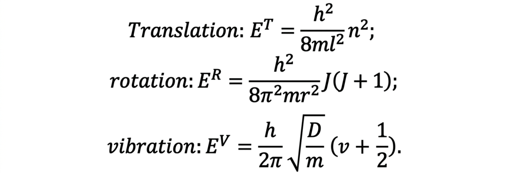
as in Jungermann, 2006
where h is Planck’s constant, m is the particle mass, l is the uncertainty of the position, r is the distance from the rotation axes, D is a force constant, n, J, v are quantum numbers.
Although the quantum numbers determine the specific energy state occupied by a molecule, the spacing between adjacent energy levels is primarily determined by the physical parameters appearing in these equations, such as mass, intermolecular forces, and molecular geometry. Jungermann’s Mass Rule and Force Rule can therefore be understood directly from these relationships. The Mass Rule follows from the fact that the particle mass appears in the denominator of the translational and rotational energy expressions.
The Force Rule can also be understood from these equations. In the expression for translational energy, the uncertainty in position, l, appears in the denominator. For example, gas molecules at low pressure experience weak intermolecular forces and therefore have a larger positional uncertainty. This increases the value of l, decreases the spacing between adjacent translational energy levels, and allows more energy levels to be occupied, leading to higher entropy. A similar qualitative relationship is observed for rotational motion, where weaker constraints on molecular rotation also reduce the spacing between rotational energy levels.
Thus, although translational, rotational, and vibrational motions have different mathematical expressions, they all exhibit the same qualitative behavior: larger masses and weaker confining forces reduce the spacing between energy levels, increase the number of accessible energy states, and therefore increase entropy.
4. Entropy as a physical property
The shelf model provides a physical interpretation of entropy by relating it to the number of accessible and occupied molecular energy levels. Unlike many thermodynamic quantities, molar entropy is an absolute property, with its zero defined at 0 K by the Third Law of Thermodynamics. Although absolute zero cannot be reached in practice, it serves as the reference point for the entropy scale. Like density, molar entropy is an intrinsic physical property of a substance that depends on temperature and reflects its molecular energy-level structure.
According to the Boltzmann distribution, the way thermal energy is distributed among these energy levels depends on their spacing. Substances with closely spaced energy levels can occupy more states at a given temperature, resulting in higher entropy and a greater capacity to store thermal energy. Conversely, substances with widely spaced energy levels occupy fewer states, have lower entropy, and store less thermal energy at the same temperature.
5. Application to understand atomic entropy trends
The Shelf model can be applied to understand this atomic entropy difference between different elements. For example, the standard atomic entropy of noble gases increases down the group (He: 15.17, Ne: 17.60 cal mol⁻¹ K⁻¹) and is generally higher than that of halogens in the gaseous state (F(g): 12.20, Cl(g): 13.42 cal mol⁻¹ K⁻¹). For noble gases, it can be assumed that they only exert negligible attractive forces under standard conditions. From the mass rule, we can conclude that the entropy increases within the group of noble gases. For halogens, the same conclusion can be made using the mass rule, however, due to the force of nonpolar atomic bond motion, the motion of each halogen is reduced. By the force rule, a larger force leads to smaller entropies.
6. Conclusion
Our first encounter with entropy usually comes through the Second Law of Thermodynamics, where we associate it with spontaneous processes and learn that the entropy of an isolated system tends to increase. Consequently, entropy is often viewed as something dynamic—a quantity that changes as a system evolves toward greater disorder.
The shelf model provides a complementary perspective by interpreting entropy as an absolute physical property rather than only as a measure of change. By visualizing how energy is distributed among discrete molecular energy levels, the model explains the origin of measured entropy values and the differences in entropy between substances. It therefore bridges the gap between the macroscopic concept of entropy in thermodynamics and its microscopic interpretation in statistical mechanics, making the concept more intuitive and physically meaningful.
Reference
Jungermann, A. H. (2006). Entropy and the shelf model: A quantum physical approach to a physical property. Journal of Chemical Education, 83(11), 1686–1694. https://doi.org/10.1021/ed083p1686


